 World of O News
Denmark Wins Both JEC Relay Races, Switzerland Gets the Cup. Today the Junior European Cup in Germany ended with an extremely exciting relay competition that left the decision about the winner of the nations ranking open until the very last metres. Up to ten teams fought both in the women’s ...
Read More »JEC Relay: Maps and Results